In my first semester of the double MSc at KTH (Systems, Control and Robotics), I took the Reinforcement Learning course — and it remains one of my favourites of the whole degree. I solved the two lab assignments entirely from scratch: a classic grid-world problem with full value iteration, and a Deep Q-Network trained on Lunar Lander. Both labs later grew playable browser editions, so you can try the exact algorithms live. En mi primer semestre del doble MSc en KTH (Systems, Control and Robotics) cursé Reinforcement Learning — sigue siendo de mis favoritas de todo el máster. Resolví los dos labs desde cero: un grid-world clásico con value iteration completa y una Deep Q-Network entrenada en Lunar Lander. Ambos acabaron con ediciones jugables en el navegador, para probar los algoritmos exactos en vivo.
🤖 Lab 1 — Minotaur Maze & Mountain Car🤖 Lab 1 — Minotaur Maze y Mountain Car
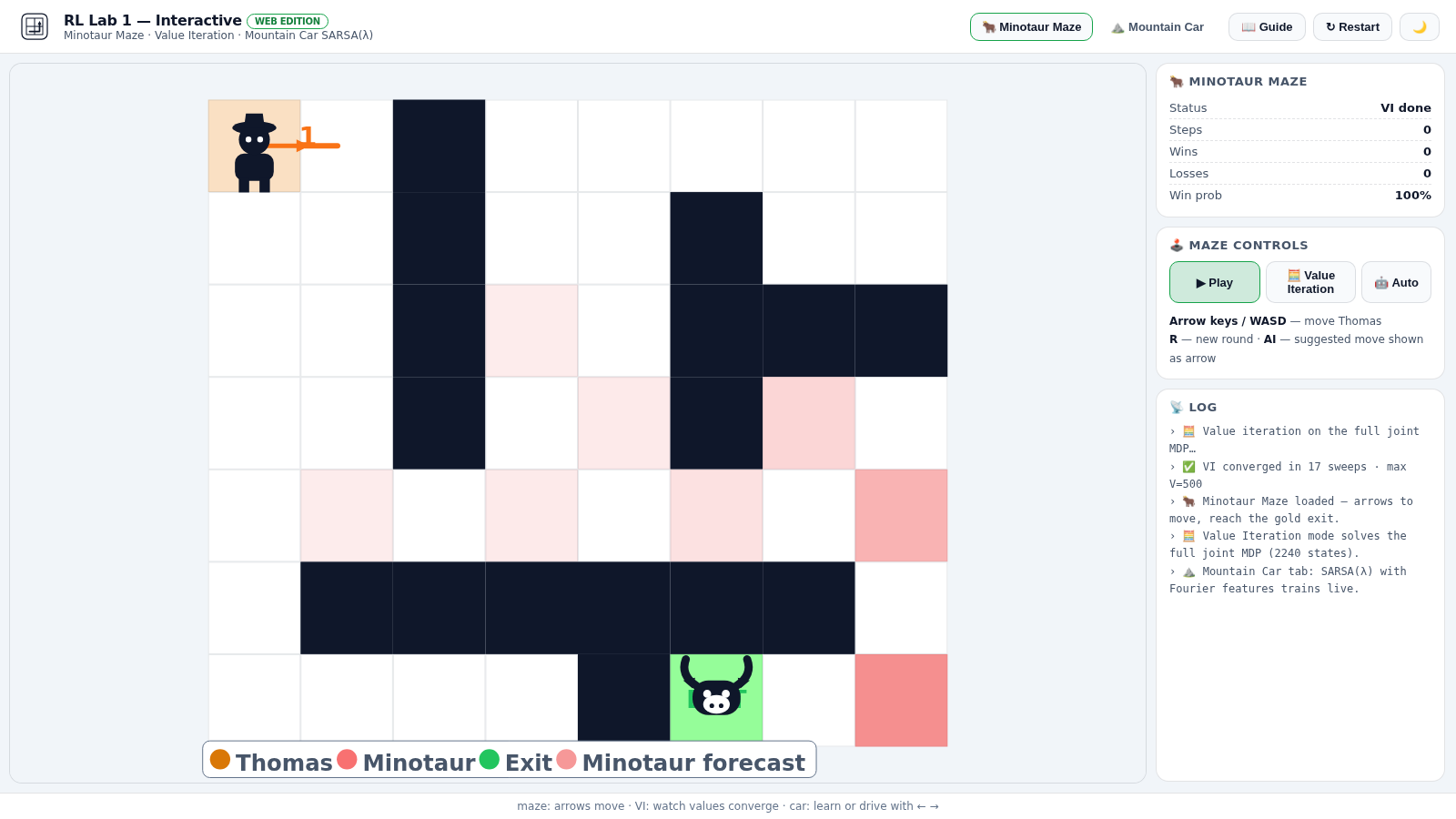
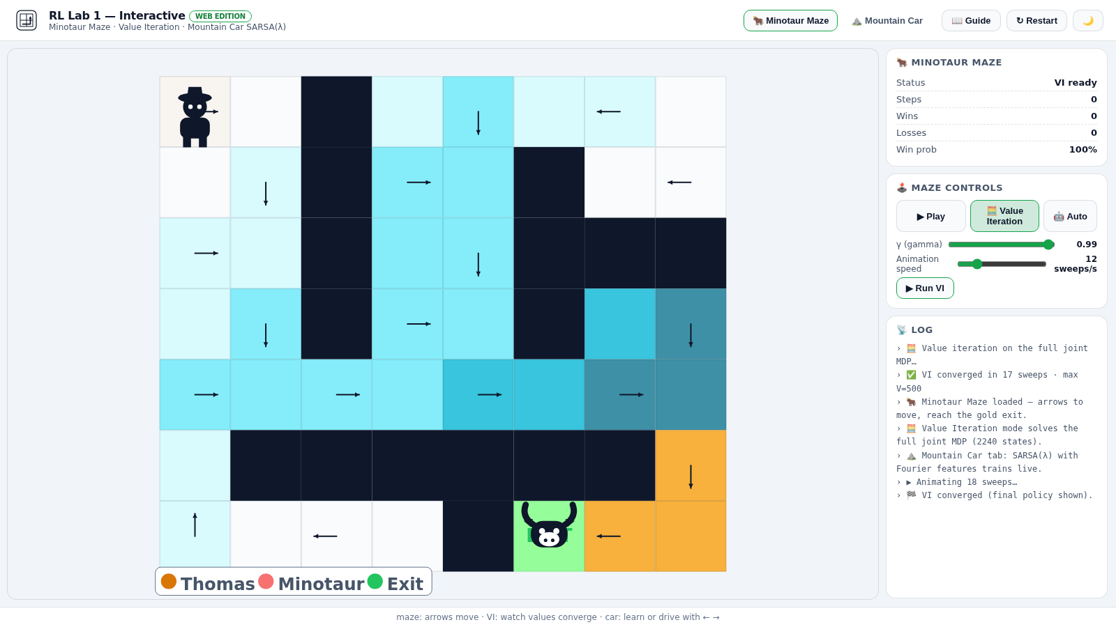
The first lab covered the fundamentals: MDPs, Bellman equations, value iteration, Q-learning and SARSA. Our first problem was the Minotaur Maze — Thomas must reach the exit while a minotaur wanders the maze. Because both agent and minotaur move, I modelled it as a joint MDP of 2,240 states and solved it with full value iteration, comparing it against Q-learning and SARSA. The web edition lets you drive Thomas yourself while an AI arrow shows what the optimal policy would do at every step, and a live heatmap visualises the V-values converging sweep by sweep: El primer lab cubrió los fundamentos: MDPs, Bellman equations, value iteration, Q-learning y SARSA. Nuestro primer problema fue el Minotaur Maze — Thomas debe llegar a la salida mientras un minotauro deambula por el laberinto. Como ambos se mueven, lo modelé como un joint MDP de 2,240 estados y lo resolví con full value iteration, comparándolo con Q-learning y SARSA. La edición web te deja mover a Thomas mientras una AI arrow muestra qué haría la política óptima en cada paso, y un heatmap en vivo visualiza los V-values convergiendo sweep a sweep:
The big idea, in plain words: imagine every maze position glowing with a number — how good it is to be there — with the exit glowing +500 and being caught −1000. Value iteration spreads that glow through the maze like water finding its level, until each position knows its best move’s promise minus the cost of moving; then the arrows simply point to the brightest neighbour. Formally, the maze is a stochastic shortest-path MDP whose state is the joint configuration of both agents, \(\mathcal{S} = \{(t_i, t_j, m_i, m_j, k)\}\), and the transition model over the minotaur’s uniformly random moves is \[ P(s' \mid s, a) = \frac{1}{|A_{\text{mino}}(s)|} \] with rewards \(+500\) for escaping and \(-1000\) for being caught. La idea, en palabras simples: imagina cada posición del laberinto con un número brillando — cuánto vale estar ahí — la salida brilla +500 y ser atrapado −1000. Value iteration propaga ese brillo como el agua buscando su nivel, hasta que cada posición conoce su mejor movimiento menos su coste; las flechas apuntan al vecino más brillante. Formalmente, el laberinto es un stochastic shortest-path MDP cuyo estado es la configuración conjunta de ambos agentes, \(\mathcal{S} = \{(t_i, t_j, m_i, m_j, k)\}\), y la transición sobre los movimientos uniformemente aleatorios del minotauro es \[ P(s' \mid s, a) = \frac{1}{|A_{\text{mino}}(s)|} \] con rewards \(+500\) por escapar y \(-1000\) por atrapar.
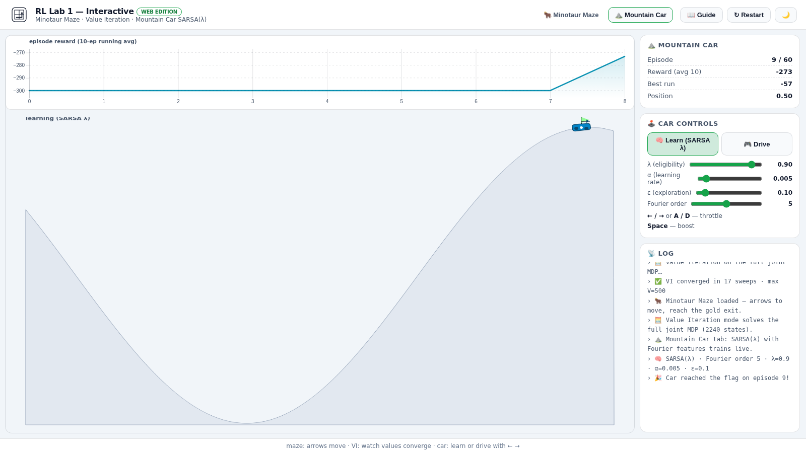
The second problem was the classic Mountain Car: a weak car that must climb a steep hill by building momentum. Here we implemented SARSA(λ) with a Fourier linear basis, eligibility traces and Nesterov momentum — a great lesson in how function approximation turns tabular algorithms into continuous-state learners: El segundo problema fue el clásico Mountain Car: un coche débil que sube una cuesta empinada acumulando momentum. Implementamos SARSA(λ) con Fourier linear basis, eligibility traces y Nesterov momentum — una gran lección de cómo la function approximation convierte algoritmos tabulares en aprendices continuos:
🤖️ Lab 2 — Deep Q-Network on Lunar Lander🤖️ Lab 2 — Deep Q-Network en Lunar Lander
The second lab jumped to deep reinforcement learning: a DQN trained from scratch (PyTorch) on LunarLander-v2 from OpenAI Gym — an 8 → 64 → 64 → 4 network with experience replay (L = 16,384 transitions), a target network updated every C = L/N = 256 steps, mini-batches of 64 and ε-greedy exploration decaying from 0.99. I ran a proper ablation study — discount factor (γ = 0.5 / 0.99 / 1.0), training length (500 / 1000 / 2000 episodes) and DQN vs. random baselines — and saved the trained models. El segundo lab saltó al deep reinforcement learning: un DQN entrenado desde cero (PyTorch) en LunarLander-v2 de OpenAI Gym — una red 8 → 64 → 64 → 4 con experience replay (L = 16,384), un target network actualizado cada C = L/N = 256 pasos, mini-batches de 64 y ε-greedy decayendo desde 0.99. Hice un ablation study serio — discount factor (γ = 0.5 / 0.99 / 1.0), duración del training (500 / 1000 / 2000 episodios) y DQN vs. baselines random — y guardé los modelos entrenados.
The big idea, in plain words: the lander learns by replaying memories — it stores what it experienced (situation → action → outcome) and practices on random memories between flights, like a pilot studying past landings. The optimal action-value function satisfies the Bellman equation \[ Q^*(s,a) = \mathbb{E}\!\left[\, r + \gamma \max_{a'} Q^*(s',a')\, \right] \] and the network \(Q(s,a;\theta)\) approximates it by minimising the TD loss \[ \mathcal{L}(\theta) = \mathbb{E}\!\left[\left( r + \gamma \max_{a'} Q(s',a';\theta^-) - Q(s,a;\theta) \right)^2\right] \] against a frozen copy \(\theta^-\) of the network — the target network keeps the scoreboard stable enough to learn from, while \(\varepsilon\)-greedy exploration occasionally presses a random button so the lander discovers moves it would never try otherwise. La idea clave, en palabras simples: el lander aprende repasando memorias — guarda lo vivido (situation → action → outcome) y practica con memorias aleatorias entre vuelos, como un piloto que estudia aterrizajes pasados. La optimal action-value function cumple la Bellman equation \[ Q^*(s,a) = \mathbb{E}\!\left[\, r + \gamma \max_{a'} Q^*(s',a')\, \right] \] y la red \(Q(s,a;\theta)\) la aproxima minimizando el TD loss \[ \mathcal{L}(\theta) = \mathbb{E}\!\left[\left( r + \gamma \max_{a'} Q(s',a';\theta^-) - Q(s,a;\theta) \right)^2\right] \] contra una copia congelada \(\theta^-\) de la red — el target network mantiene el marcador estable para poder aprender, mientras la exploración \(\varepsilon\)-greedy pulsa a veces un botón al azar para que el lander descubra movimientos que nunca probaría.
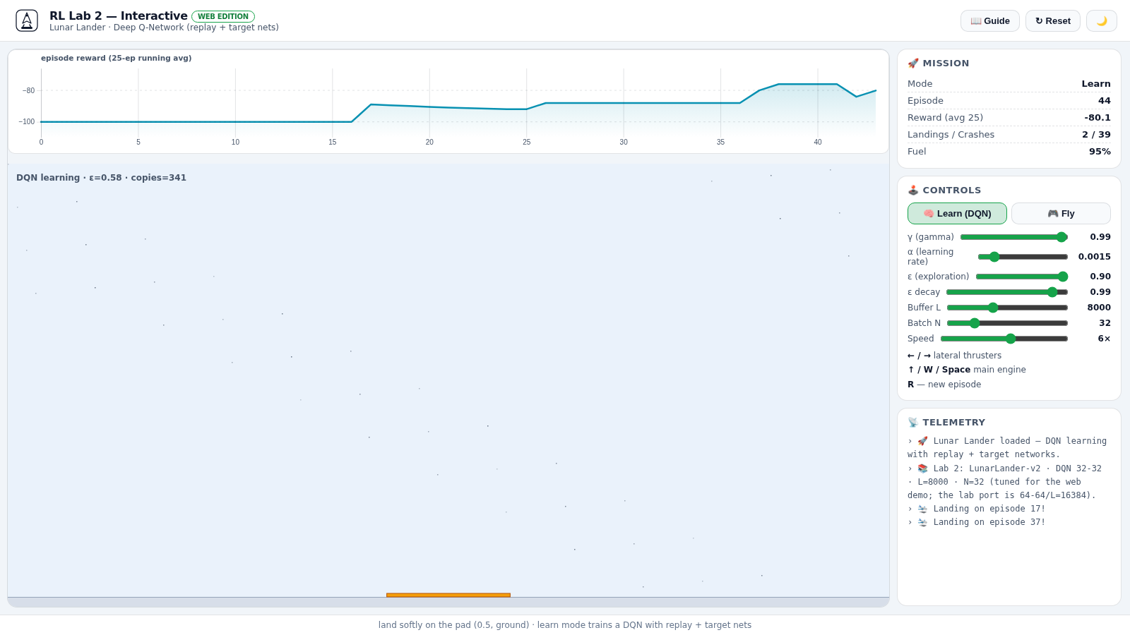
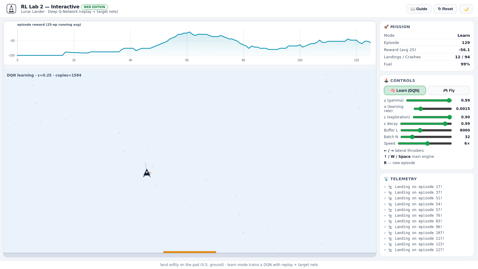
The web edition is the fun part: Learn mode trains the DQN live in your browser with adjustable hyperparameters (γ, α, ε, decay, replay buffer, batch size and speed), plotting the running reward and logging every landing; Fly mode hands you the thrusters: La edición web es lo mejor: el Learn mode entrena el DQN en vivo en el navegador con hyperparameters (γ, α, ε, decay, replay buffer, batch size, speed), graficando la running reward y registrando cada aterrizaje; el Fly mode te da los thrusters:
🎮 Play both labs in the browser🎮 Juega los labs en el browser
Both labs are deployed on GitHub Pages — the JavaScript cores are 1:1 ports of the Python code (same state
space, same Bellman backups, same replay buffer) with matching node:test suites:
Ambos labs están en GitHub Pages — los núcleos JavaScript son ports 1:1 del código Python (mismo state
space, mismos Bellman backups, mismo replay buffer) con suites node:test iguales:
- RL Lab 1 — Minotaur Maze + Value Iteration + Mountain CarRL Lab 1 — Minotaur Maze + Value Iteration + Mountain Car
- RL Lab 2 — train the DQN or fly the lander yourselfRL Lab 2 — entrena el DQN o vuela el lander
🎓 What the course gave me🎓 Lo que me dio el curso
- MDP thinking: modelling sequential decisions — states, actions, rewards, and the Bellman backup — is now second nature.
- MDP thinking: modelar decisiones secuenciales — states, actions, rewards y el Bellman backup — ya es algo natural.
- The tabular → deep bridge: SARSA(λ) with Fourier features in Lab 1, DQN with replay and target nets in Lab 2 — the same ideas, scaled up.
- Puente tabular → deep: SARSA(λ) con Fourier features en Lab 1, DQN con replay y target nets en Lab 2 — las mismas ideas, a mayor escala.
- Deep-RL stability toolkit: experience replay, target networks, ε decay — and the discipline of ablating each one to see it matter.
- Deep-RL stability toolkit: experience replay, target networks, ε decay — y la disciplina de ablacionar cada uno para verlo.
- Experiment hygiene: every run logged, every model saved, every figure labelled — the habit that made the labs reproducible (and later, ported to the browser).
- Experiment hygiene: cada run logueado, cada modelo guardado, cada figura rotulada — el hábito que hizo los labs reproducibles (y luego portados al navegador).
GitHub · rl_lab1GitHub · rl_lab1 GitHub · rl_lab2GitHub · rl_lab2 Play Lab 1Play Lab 1 Play Lab 2Play Lab 2 KTH · Systems, Control and RoboticsKTH · Systems, Control and Robotics PyTorch · OpenAI Gym · SARSA(λ) · DQNPyTorch · OpenAI Gym · SARSA(λ) · DQN