For the SCON course (Sistemas de Comunicación) in the UPM master’s programme, I built a complete analysis of my own home WiFi network: a beacon scanner that captured real over-the-air traffic, a per-room signal study of all 26 rooms of the flat, band occupancy statistics for 2.4/5 GHz, and two simulations — optimal router placement and WiFi repeater placement — built on a path-loss model fitted from my own measurements. Para el curso SCON (Sistemas de Comunicación) del máster en UPM, construí un análisis completo de mi red WiFi doméstica: un beacon scanner de tráfico real over-the-air, un estudio de la señal por habitación en las 26 estancias, ocupación de bandas para 2.4/5 GHz, y dos simulaciones — colocación óptima de router y repetidor WiFi — con un path-loss model ajustado con mis mediciones.
📡 The pipeline📡 El pipeline
wifi_scanner.py — a scapy-based monitor-mode scanner: it hops channels (1 → 14 →
36 → 60) and records every beacon — BSSID, SSID, zone, dBm, channel, crypto — into a CSV.
DomesticNetworkAnalysis.ipynb — the full analysis: a choropleth of the measured
5 GHz signal per room, 2.4/5 GHz band occupancy and channel statistics, and the placement
simulations. analysis_model.py — the signal model extracted from the notebook into a
reusable, unit-tested module (and later ported 1:1 to JavaScript for the web edition).
wifi_scanner.py — un scanner monitor-mode con scapy: salta entre canales (1 → 14 →
36 → 60) y guarda cada beacon — BSSID, SSID, zone, dBm, channel, crypto — en un CSV.
DomesticNetworkAnalysis.ipynb — el análisis completo: un choropleth de la señal
5 GHz por habitación, ocupación de bandas 2.4/5 GHz y estadísticas de canal, y las simulaciones
de colocación. analysis_model.py — el signal model extraído del notebook a un
módulo reutilizable con unit tests (y luego portado 1:1 a JavaScript para la web).
📈 What the scan showed📈 Qué mostró el scan
The measured 5 GHz heatmap tells a very familiar story: the router lives in Habitación 1 (strongest mean signal, around −39 dBm), and the signal degrades steadily through the hallway into the living room, terrace, bathrooms and — the weakest corner of the flat — the kitchen (−86 dBm). The band-occupancy analysis completes the picture with channel usage across the whole building: El heatmap medido de 5 GHz cuenta una historia conocida: el router vive en Habitación 1 (señal media más fuerte, unos −39 dBm), y la señal va degradándose por el pasillo hacia el salón, la terraza, los baños y — la esquina más débil del piso — la cocina (−86 dBm). La ocupación de bandas completa el cuadro con el uso de canales en todo el edificio:
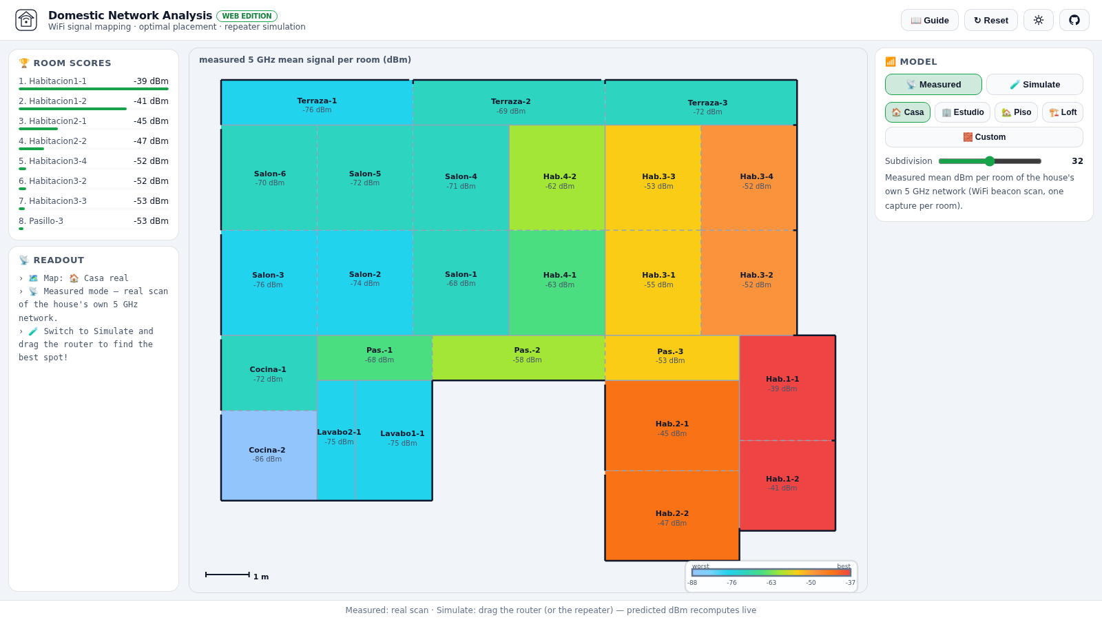
Measured mode — the real 5 GHz scan of the house’s own network, per room, with the metre scale bar at the bottom.Measured mode — el scan real de 5 GHz de la red de casa, por habitación, con la barra de escala en metros abajo.
📡️ The model and the simulations📡️ Modelo y simulaciones
The core of the project is a simple, interpretable path-loss model fitted from the real measurements. The predicted received power at distance \(d\) metres from the router, through \(W\) walls: El núcleo del proyecto es un path-loss model simple e interpretable, ajustado con las mediciones reales. La potencia recibida predicha a \(d\) metros del router, a través de \(W\) paredes:
\[ P(d) = P_{\max} - 3\,d - 7\,W \]i.e. 3 dB/m free-space-ish attenuation plus 7 dB per interior wall, with \(P_{\max} = -39.2\) dBm calibrated from the measurements — the notebook’s exact model, with a hand-built 10×10 wall matrix between the house zones and a zone-weighted score (living areas matter more). The web edition refines that matrix: every heatmap cell walks the straight line from the router and counts the actual walls crossed by ray-casting — including the exterior walls when the line leaves the house through a concave corner or notch, with the travelled distance split into its in-flat and out-of-flat parts, both charged in the distance degradation — so neighbouring rooms never lose to more distant ones and corner rooms don’t over-score. es decir, atenuación free-space-ish: 3 dB/m más 7 dB por pared interior, con \(P_{\max} = -39.2\) dBm calibrado con las medidas — el modelo exacto del notebook, con una wall matrix 10×10 manual entre las zonas de la casa y un score ponderado por zona (pesan más las zonas de estar). La edición web refina esa matriz: cada celda recorre la línea recta desde el router y cuenta las paredes cruzadas por ray-casting — incluidas las exteriores cuando la línea sale por una esquina cóncava o un hueco, con la distancia dividida en sus partes dentro y fuera del piso, ambas contadas en la degradación de distancia — así las vecinas nunca pierden frente a las más lejanas y las esquinas no puntúan de más.
All distances are converted to real metres with the geojson scale factor ×4.45 (the original flat is ~120 m² — 14.2 × 10.4 m — so e.g. the Salon-6 → Habitacion2-2 line is 11.8 m), and every map carries a scale bar showing the real size at a glance: Todas las distancias pasan a metros reales con el geojson scale factor ×4.45 (el piso original tiene ~120 m² — 14.2 × 10.4 m — la línea Salon-6 → Habitacion2-2 mide 11.8 m), y cada mapa lleva una scale bar con el tamaño real de un vistazo:
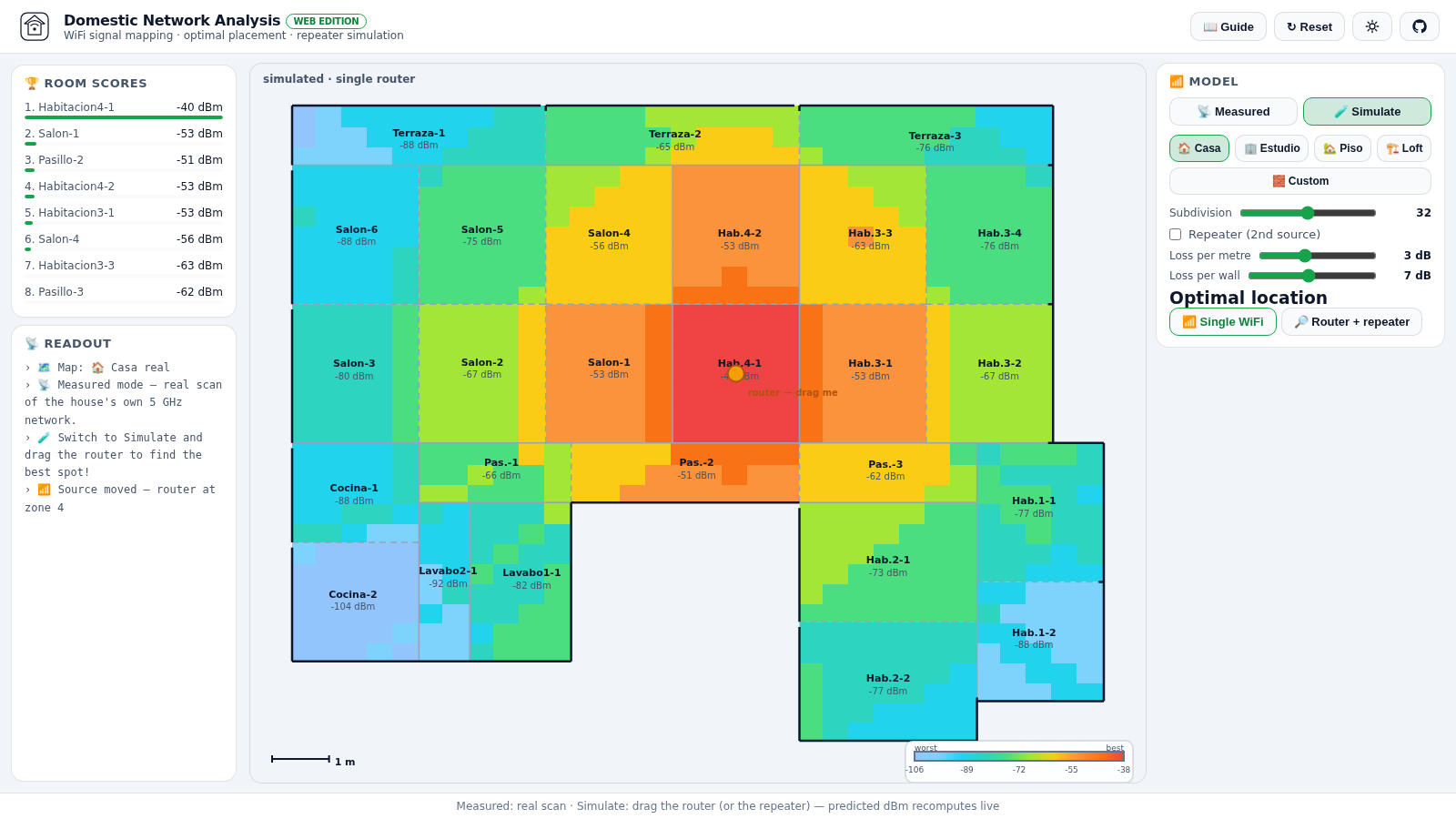
Simulate mode — drag the router (and a repeater) anywhere; every cell’s predicted dBm, the score ranking and the heatmap recompute live.Simulate mode — arrastra el router (y un repetidor) donde sea; el dBm de cada celda, el ranking y el heatmap se recalculan en vivo.
Two solvers run the exhaustive placement search over every room: Dos solvers ejecutan la búsqueda exhaustiva en cada habitación:
- the single-WiFi search — every room as the candidate router location;
- el single-WiFi search — cada habitación como candidata a router;
- the router + repeater search — brute-forces every room-center pair, with each cell served by the stronger of the two paths.
- el router + repeater search — por fuerza bruta en cada par de centros, sirviendo cada celda por la ruta más fuerte.
In the current capture the two-device search leads the scoreboard with Pasillo-2 at −39 dBm — the central hallway, the classic spot, now with a second source covering the corners the single router can’t reach: En esta captura, el two-device search lidera el marcador con Pasillo-2 a −39 dBm — el pasillo central, el lugar clásico, y una segunda fuente cubre las esquinas que el router solo no alcanza:
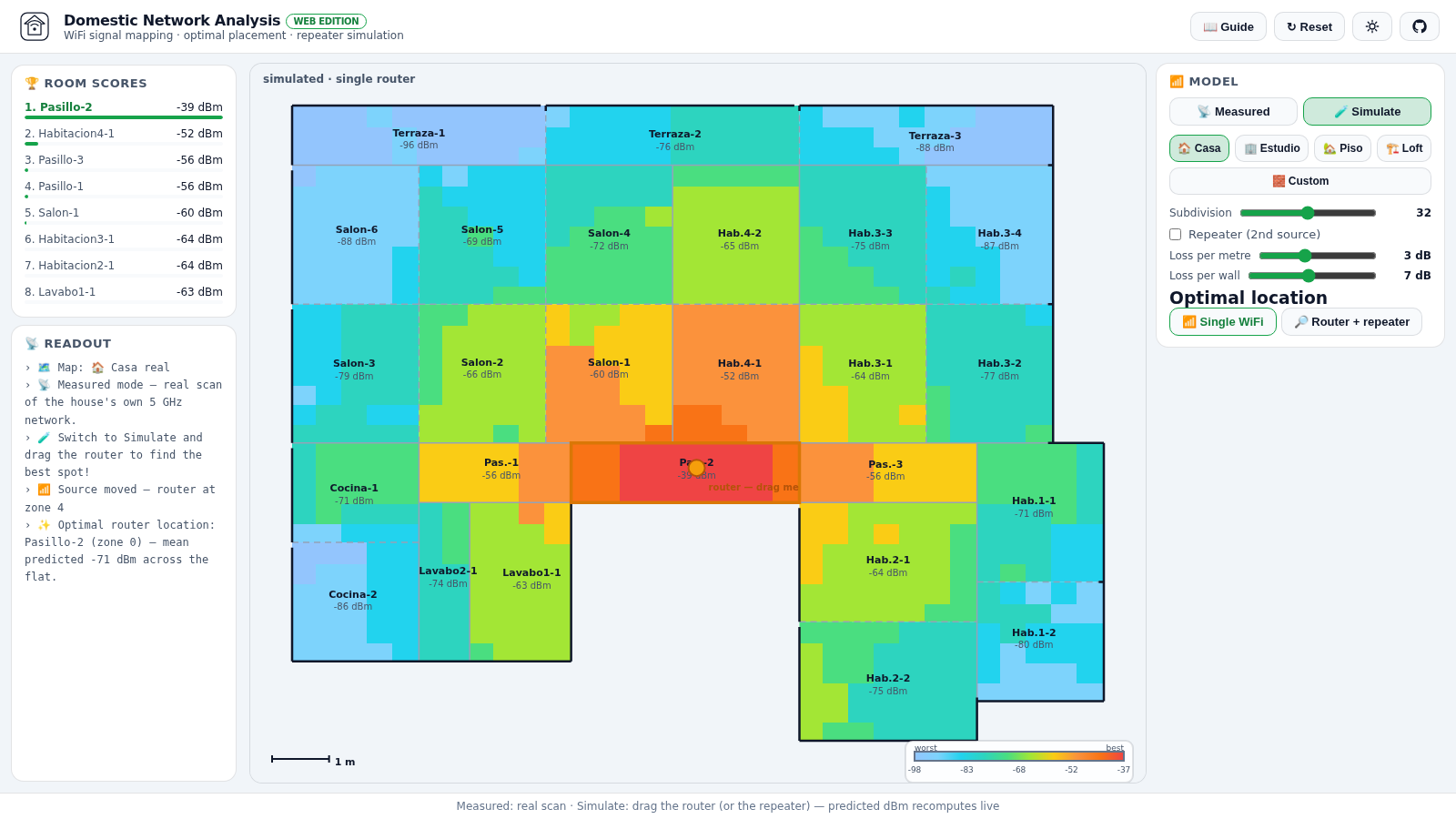
Optimal placement — the router + repeater search, with Pasillo-2 leading the scoreboard at −39 dBm.Optimal placement — el router + repeater search, con Pasillo-2 liderando el marcador a −39 dBm.
🎮 Try it in the browser🎮 Juega en el navegador
The whole lab is playable at alejp1998.github.io/domestic_net_analysis: Todo el lab es jugable en alejp1998.github.io/domestic_net_analysis:
- 4 flat plans — the real scanned home (rebuilt as a perfectly tiled, gap-free plan) plus three designed flats: Estudio, Piso 2 hab, Loft;
- 4 flat plans — la casa escaneada (plano reconstruido, teselado y sin huecos) y tres pisos diseñados: Estudio, Piso 2 hab, Loft;
- discrete subdivision model — a slider chooses the cell size; every cell predicts its own signal, so heatmaps are smooth and walls are grid-aligned;
- discrete subdivision model — un slider elige el cell size; cada celda predice su señal, con heatmaps suaves y paredes alineadas al grid;
- measured — the real scan heatmap per room; simulate — drag the router (and a repeater) with live recomputation and dB/metre + dB/wall sliders; find optimal room — single-WiFi or router + repeater;
- measured — el heatmap real por habitación; simulate — arrastra el router (y un repetidor), recálculo en vivo y sliders dB/metro + dB/pared; find optimal room — single-WiFi o router + repeater;
- scale bar on every map — the real size at a glance, from the ×4.45 geojson factor;
- scale bar en cada mapa — tamaño real de un vistazo, del factor geojson ×4.45;
- custom flat editor — a separate left-hand panel lets you paint your own rooms on a 1 m² grid, name and zone them, and analyze them with the full simulation:
- custom flat editor — un panel a la izquierda te deja pintar tus habitaciones en un grid de 1 m², nombrarlas, zonificarlas y analizarlas con la sim completa:
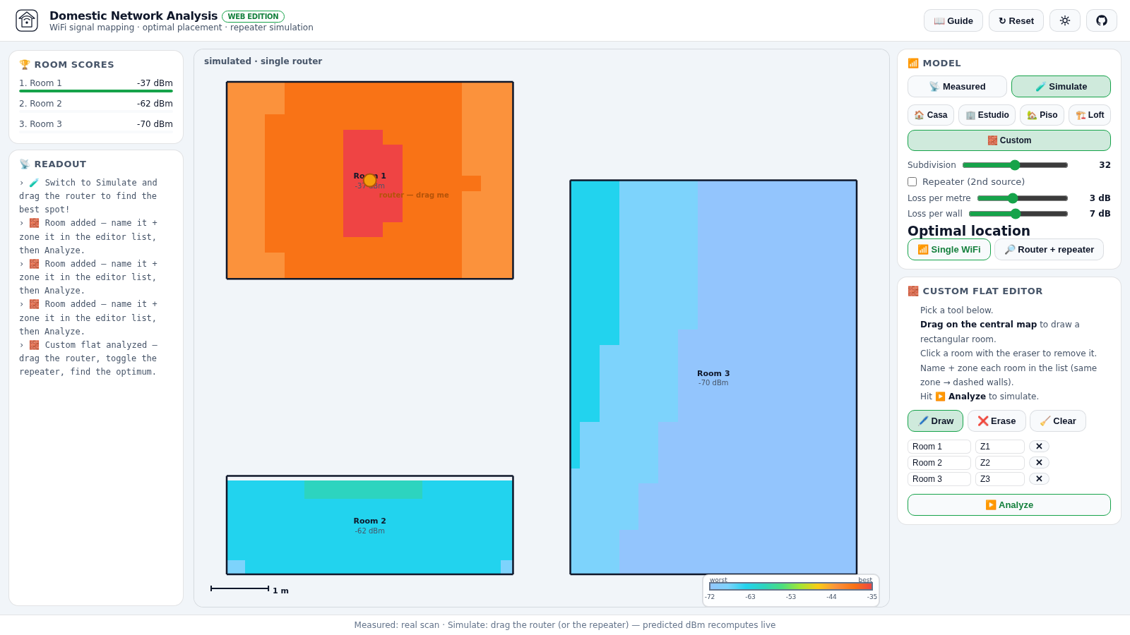
Custom flat editor — paint rooms on a 1 m² grid, name and zone them, and analyze with the full sim.Custom flat editor — pinta habitaciones en grid 1 m², nómbralas, zonifícalas, analiza con la sim.
The JavaScript model port is cross-checked against the Python — the unit-tested analysis_model.py
suite (6/6 tests) keeps both honest.
El port JavaScript del modelo se contrasta con Python — la suite con unit tests de analysis_model.py
(6/6) los mantiene honestos.